The IPCC TAR [2001] Spaghetti Diagram

Post-1960 values of the Briffa MXD series are deleted from the IPCC TAR multiproxy spaghetti graph. These values trend downward in the original citation (Briffa [2000], see Figure 5), where post-1960 values are shown. The effect of deleting the post-1960 values of the Briffa MXD series is to make the reconstructions more "similar". The truncation is not documented in IPCC TAR. In most cases, people would ask: who at IPCC truncated this series? why did they do so? who approved the truncation? what process was involved in approving the truncation? I've gone through a laborious process to calculate what the untruncated IPCC spaghetti graph would look like and show the calculations here.

Figure 1 below from IPCC here  http://www.grida.no/climate/ipcc_tar/wg1/fig2-21.htm http://www.grida.no/climate/ipcc_tar/wg1/images/fig2-21.gif  shows the Brifa MXD, together with Jones98, MBH99 and CRU instrumental. The green line showing Briffa MXD reaches a low around 1620, another low around 1690, rises to around 1800, a low around 1820 and then rises in steps. Around 1900, it has a little low, but is higher than the other series (as in the late 19th century), merging in the general graphic from about 1920 to 1950. 

Figure 1. IPCC TAR Figure 2-21. The line in green is the Briffa MXD (density) reconstruction. Original caption: Figure 2.21: Comparison of warm-season (Jones et al., 1998) and annual mean (Mann et al., 1998, 1999) multi-proxy-based and warm season tree-ring-based (Briffa, 2000) [QSR] millennial Northern Hemisphere temperature reconstructions. The recent instrumental annual mean Northern Hemisphere temperature record to 1999 is shown for comparison. Also shown is an extra-tropical sampling of the Mann et al. (1999) temperature pattern reconstructions more directly comparable in its latitudinal sampling to the Jones et al. series. The self-consistently estimated two standard error limits (shaded region) for the smoothed Mann et al. (1999) series are shown. The horizontal zero line denotes the 1961 to 1990 reference period mean temperature. All series were smoothed with a 40-year Hamming-weights lowpass filter, with boundary constraints imposed by padding the series with its mean values during the first and last 25 years.

For someone looking at the graphic below, it looks like it turns up in the late 20th century parallel to the instrumental graph. But appearances can be deceptive. Here is a blow-up of the image in the 20th century. You can discern the green Briffa MXD with a slight downturn. If you don't look closely, it looks like it continues upward, but the upward turn is from one of the two Mann series. The end of the green Briffa MXD series seems to be about 1960 - just before the 1961-1990 base period and is shown as ending at a level of ~0.02 deg C (1961-90 reference).  The series goes just above the 1961-1990 reference line, a maximum of ~0.03 deg C. How does this compare to original references?

Figure 2. Blowup of IPCC TAR Figure 2-21.

First Reference: Briffa [QSR 2000]

Figure 3 below shows the Briffa MXD series from Briffa [QSR 2000], cited above. There are two versions illustrated here: black - NHD1 (also shown in Nature 1998) and green- LFD. The shape of the green LFD series is quite similar to the shape of the IPCC TAR Briffa MXD version.I have not been able to locate the basis of smoothing, but Briffa often uses 25-year gaussian smoothing and the shape looks consistent with that (see more below).   It looks a little less smoothed than the IPCC TAR version (which has 40 year smoothing). There is no digital archive for this article. There is an archive of the NHD1 series at WDCP in connection with Briffa et al [Nature 393, 1998], but I have not located any archive of the LFD series.   The caption asserts that the temperature scale (right-hand) applies only to the NHD1 version, while the left-hand scale in standard deviation units applies to the LFD version. The calibration of the NHD1 series to temperature is not described here (See Nature 1998). The temperature scale is not provided in QSR 2000, but, based on the archive for Briffa et al.1998a [Nature 393], is 1881-1960. This would require a deduction of 0.236 deg C to a 1961-1990 reference period.  The thick black line shows a spliced instrumental series starting ~1880 [why not 1850s?]

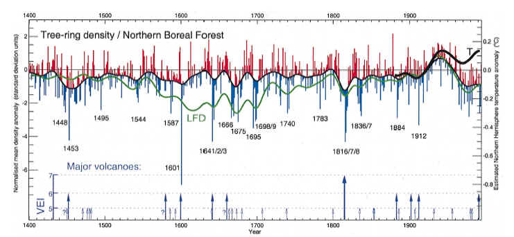
Figure 3. Taken from Figure 5, Briffa [QSR 2000]  Original caption:  An indication of growing season temperature changes across the whole of the northern boreal forest. The histogram indicates yearly averages of maximum ring density at nearly 400 sites around the globe, with the upper curve highlighting multidecadal temperature changes. Extreme low density values frequently coincide with the occurrence of large explosive volcanic eruptions, i.e. large values of the Volcanic Explosivity Index (VEI) shown here as arrows (see Briffa et al., 1998a). The LFD curve indicates low-frequency density changes produced by processing the original data in a manner designed to preserve long-timescale temperature signals (Briffa et al., 1998c [Roy.Soc.]). Note the recent disparity in density and measured temperatures (¹) discussed in Briffa et al., 1998a [Nature 393], 1999b [Nature 391]). Note that the right hand axis scale refers only to the high-frequency density data.

The NHD1 series is "an average timeseries of all of the density chronologies (NHD1)", while the LFD series is age-banded averaging, i.e. " first, only within specific tree age bands, and then combining these to produce an average timeseries in which the potential sample age bias discussed earlier is removed, but long timescale information is preserved (Briffa et al., 1998c [Roy Soc]). . In both the NHD1 and LFD versions, the density reconstruction in the 2nd half 20th century falls to very low levels - otherwise characteristic of cold periods in the 17th century and early 19th century. This is commented on by Briffa here (and elsewhere), who is unable to account for this, hypothesizing some "unknown anthropogenic" cause. 

So there are several questions at this stage:

1. If the IPCC TAR spaghetti diagram uses this LFD series, how is it scaled (since the series in the citation does not justify the scaling in the spaghetti graph)?

2. What does the spaghetti graph look like if the post-1960 LFD series is included with the diagram? 

Answering this has not proven easy.

Second Reference: Briffa et al., 1998c  [Roy. Soc.]

Briffa et al. 1998c [Roy. Soc.] is cited in Briffa [QSR 2000], but it does not contain a derivation of the LFD density series. In connection with this MXD data, Briffa et al. 1998c contains only the following figure, which appears to replicate the NHD1 series shown in QSR 2000 Figure 5, rather than the LFD series. However, the illustrated period begins ~1600 rather than ~1400 as in the QSR [2000] figure. It is shown in standard deviation units, rather than being calibrated to temperature, so it does not answer question 1 or 2.

Figure 4. Taken from Briffa et al. 1998c [Roy. Soc.] Figure 5. Original Caption: Series of annual and decadally smoothed standardized anomalies (1901-70 base) of tree-ring density averaged across all sites shown in Figure 1. The dotted lines are +-1 s.d. about the long-term mean. The extreme negative departures often coincide with the eruption dates of known explosive volcanoes.

Briffa et al., 1998c [Roy. Soc.] discusses problems in tree-ring standardization, noting many difficulties in going from high-frequency results to centennial results based on tree rings, mentioning RCS methods as a proposed means of capturing low-frequency changes, when there is sufficient replication. They also note difficulties because of "anomalous" density behaviour in the 20th century,

The RCS method potentially provides much more information on century-to-century time-scale changes in temperatures than the previous approach, but the lack of very long temperature data means that it is simply not possible to verify this centennial time-scale information without reference to other evidence (Briffa et al. 1995) [Nature - Polar Urals]. Tree rings (TRW and MXD data) provide demonstrably accurate information on interannual and decadal time-scales, but it is clear that as we try to deduce centennial and longer scales of information, the reconstructions are subject to increasing levels of uncertainty. Nevertheless, where good data replication exists, especially if many samples from a wide range of tree ages are available over long periods, the single RCS approach can be used to attempt to capture long, as well as short, time-scale information...

On annual, decadal, and probably even centennial time-scales, tree-ring data are demonstrably reliable palaeoclimate indicators, but where the focus of attention shifts to inferences on century and longer time-scales, the veracity of inferred change is difficult to establish. Furthermore, recent analyses of large regional-scale growth patterns and absolute tree growth changes over recent centuries strongly suggest that anthropogenic influences are increasingly challenging our assumptions of uniformitarianism in tree growth-climate responses.

Third Reference: WDCP Archive for Briffa et al. 1998a [Nature 393] 

There is a WDCP archive for Briffa et al. [1998a, Nature 393] at ftp://ftp.ncdc.noaa.gov/pub/data/paleo/treering/reconstructions/n_hem_temp/nhemtemp_data.txt  (July 15, 2003). The archive states: 

The data consists of two timeseries representative of Northern Hemisphere growing season temperatures for the period 1400-1994, derived from means of 383 maximum latewood density chronologies from the northern Boreal forest. Both series are given in dimensionless standardised anomalies, and one has also been rescaled to give an estimate of Northern Hemisphere land and marine temperature anomalies.

The timeseries are:

NHD1 (dimensionless) Two-stage average of Northern Hemisphere maximum latewood density tree-ring chronologies.
NHLMT (degrees Celsius anomalies, with respect to the 1881-1960 mean) Estimate of Northern Hemisphere land and marine growing-season (April-September) temperature anomalies based on NHD1.
NHD2 (dimensionless) One-stage average of Northern Hemisphere maximum latewood density tree-ring chronologies.

The correlation between NHD1 and the anomaly series is almost exactly 1, showing that the anomaly series is thus just a re-scaled version of NHD1. All three series are zeroed on 1881-1960. The standard deviations of the two normalized series are 1 for the 1881-1960 period (confirming 1881-1960 normalization). The standard deviation for the anomaly series is 0.117 deg C (about 50% of the corresponding CRU standard deviation of  0.236 deg C).  The anomaly version appears visually identical with QSR 2000 Figure 5 - the 1601 downspike is about minus 0.8σ in both cases.  

Figure 5. Plot of data at Briffa et al 1998a WDCP archive. Top - NHD1; middle - anomaly derived from NHD1; bottom - NHD2.

None of this assists in the two questions: scaling the LFD series to temperature and demonstrating the effect of the LFD truncation in the IPCC TAR diagram.

Fourth Reference: Briffa et al. [JGR, 2001] and its WDCP Archive

Continuing the search for a source for the Briffa MXD series in IPCC TAR, I turn now to Briffa et al. [JGR 2001], together with its archive at WDCP, which has two differently scaled versions of what appear to be variations of the LFD series. The shape of Figure 6 below is fairly similar to the LFD version in QSR 2000.  It's hard to tell whether the differences pertain to different smoothing or to differences in the underlying series. No digital versions are available for either QSR Figure 5 LFD or JGR 2001 Figure 6. The instrumental temperature version goes from ~1870-1880 to the present: you can more or less the intersection of the two curves. The reference scale is 1961-1990, which is about 0.24 deg C higher than the 1881-1960 reference period of QSR Figure 5. The minimum smoothed low of Figure 6 is ~0.9 deg C in the lows of the 1670s and ~1700, while the smoothed high is about 0.15 deg C around 1937. The low values in the late 20th century are shown here and are noted once more in the running text (without giving any explanation). 

Figure 6. Figure 6 from Briffa et al [JGR 2001] Original caption: Figure 6. The 25-year smoothed age-banded reconstruction of the ALL temperature series, combined with the 25-year high-pass filtered variability from the "Hugershoff standardized" reconstruction [Briffa et al., 1998a], the latter shown as annual bars above and below the 25-year variations. The thin smooth curve shows the 25-year smoothed Hugershoff standardized reconstruction. The striped curve shows the 25-year smoothed observed record.

The second rendering of this data in Briffa et al. [2001] is in the Plate 3 spaghetti graph, a small version shown below. A larger version is here http://www.ncdc.noaa.gov/paleo/pubs/briffa2001/plate3.gif . The spaghetti graph is also a 1961-1990 reference consistent with both the IPCC TAR spaghetti graph and Figure 6. The Briffa MXD series is light blue. scale is different than Figure 6, although the shape appears similar, allowing for different smoothing (25-year in Figure 6, 50 years in Plate 3.) The 17th century lows in Figure 6 are around minus 1 degree C, while in Plate 3, they are slightly above minus 0.5 deg C. (which are consistent with the lows in the IPCC spaghetti graph). However, the high for the Briffa MXD series in Figure 6 was jsut over 0.1 deg C, while here is just under 0.0 deg C (while in the IPCC TAR spaghetti graph, the maximum is slightly above 0.0). Post-1960 values are truncated in Plate 3, as in the IPCC TAR spaghetti graph, but unlike Figure 6 and WSR Figure 5.  The Plate 3 version ends at ~ minus 2 deg C, lower than the end point of the IPCC TAR diagram (~ minus 0.01 deg C).

Figure 7. Plate 3 from Briffa et al. [JGR 2001]. Original Caption: Plate 3. Comparison of six large-scale reconstructions, all recalibrated with linear regression against the 1881-1960 mean April-September observed temperature averaged over land areas north of 20N. All series have been smoothed with a 50-year Gaussian-weighted filter and are anomalies from 1961-1990 mean. Observed temperature for 1871-1997 (black) from Jones et al. (1999); circum-Arctic temperature proxies for 1600-1990 (yellow) from Overpeck et al.(1997); northern hemisphere temperature proxies for 1000-1980(red) from Jones et al. (1998); global temperature and non-temperature proxies for 1000-1980 (purple) from Mann et al. (1998, 1999); and three northern Eurasian tree ring width chronologies for 1000-1987 (green) from Briffa and Osborn (1999); 13 Northern Hemisphere temperature proxies for 1000-1987 (orange) from Crowley and Lowery (2000), but excluding the two low-resolution records used by them; and the NH reconstruction from the age-banded analysis presented in this study for 1402-1960 (blue), bounded by the 1 and 2 sigma standard errors. 

Unsmoothed data for the above diagram is archived at ftp://ftp.ncdc.noaa.gov/pub/data/paleo/treering/reconstructions/n_hem_temp/briffa2001jgr3.txt . The data for Briffa et al. [2001[ is set to NA after 1960.  The figure below is a plot of the archived data using a 50-year gaussian smooth. I've used purple for the Briffa et al [2001] reconstruction rather than light blue as above, to highlight it here.

Figure 8. Plot of smoothed (25-year) data at WDCP archive for Briffa et al [JGR 2001]. Color code as for Figure 7, other than purple for Briffa MXD series.

What is the difference in scaling between Figure 6 and Plate 3? The text in Briffa et al. [2001] says that the spaghetti graph was constructed by re-scaling, using regression of all of the various series against the 1881-1960 CRU temperature series (with an ad hoc variation for Crowley-Lowery, where some of the data was left out of the re-scaling). So there should be a linear transformation from the Figure 6 version to the Plate 3 version. If this transformation can be determined by comparing visual scales of Figure 6 to Plate 3, then the Figure 6 digital version can be estimated prior to 1960 from the archived Plate 3 version; an estimate of the post-1960 Figure 6 version to 1990 can be made by digital estimates from the print Figure 6; and re-transformed back to a Plate 3 version and then to an IPCC TAR version. 

To do so, I applied the two smoothed versions, matching the 17th century low  of ~ -0.95 in Figure 6 ( minus 0.67 in the digital Plate 3 smooth) and the 1930s high of  ~0.12 in Figure 6 ( 0.0143 in the digital Plate 3 smooth.)

Figure 9. Dashed - Plate 3 version; solid black - transformed Plate 3 version in Figure 6 scale; red - post-1960 Figure 6 values inserted by visual estimates from print version.

Following the above procedures, the post-1960 values of Figure 6 applied to the Plate 3 version are shown below in a dashed line: reaching very low levels in the 1980s (comparable to prior very cold periods.) The comparison with IPCC TAR is even more extreme, since it ends at little under the 0.0 reference point.

Figure 10. Emulation of Briffa et al [2001] Plate 3. As Figure 8, but with post-1960 values for Briffa MXD included (dashed purple) corresponding to Figure 9 above.

IPCC TAR Figure 2-21

Returning now to the original IPCC Figure, here is the Figure with the withheld Briffa MXD data, shown in dashed blue. Obviously, the withholding of the post-1960 values makes the proxies look much more in agreement than they really are. The withholding was disguised by the color scheme as shown in Figure 2 above.

Figure 11. Emulation of IPCC TAR Figure 2-21, with post-1960 values for Briffa MXD included (dashed purple). Black - MBH99, red - Jones98,  blue - Briffa MXD, orange - CRU instrumental.